


ABSTRACT
We present a new and complete library of synthetic spectra for modeling the component of emission that is reflected from an illuminated accretion disk. The spectra were computed using an updated version of our code xillver that incorporates new routines and a richer atomic database. We offer in the form of a table model an extensive grid of reflection models that cover a wide range of parameters. Each individual model is characterized by the photon index Γ of the illuminating radiation, the ionization parameter ξ at the surface of the disk (i.e., the ratio of the X-ray flux to the gas density), and the iron abundance AFe relative to the solar value. The ranges of the parameters covered are 1.2 ⩽ Γ ⩽ 3.4, 1 ⩽ ξ ⩽ 104, and 0.5 ⩽ AFe ⩽ 10. These ranges capture the physical conditions typically inferred from observations of active galactic nuclei, and also stellar-mass black holes in the hard state. This library is intended for use when the thermal disk flux is faint compared to the incident power-law flux. The models are expected to provide an accurate description of the Fe K emission line, which is the crucial spectral feature used to measure black hole spin. A total of 720 reflection spectra are provided in a single FITS file (http://hea-www.cfa.harvard.edu/~javier/xillver/) suitable for the analysis of X-ray observations via the atable model in xspec. Detailed comparisons with previous reflection models illustrate the improvements incorporated in this version of xillver.
Export citation and abstract BibTeX RIS
1. INTRODUCTION
A large number of observations in the past few decades have established the general properties of the X-ray spectra from accreting luminous sources. These are systems in which a compact object, either a neutron star or a black hole, affects the surrounding material with its vast gravitational forces, which leads to accretion of large quantities of gas and consequently to the release of large amounts of radiation, mostly in the X-ray band. The compact object can be a supermassive black hole such as those present in the active galactic nuclei (AGNs) of many galaxies, or of stellar mass, such as is the case of many galactic black holes (GBHs).
In AGNs, the X-ray continuum is usually characterized by a power-law spectrum with photon index Γ, which can typically be observed to lie in the 1.8 ≳ Γ ≳ 2.2 range, although in some extreme cases it can be either closer to 1 or larger than 3, extending to high energies with an exponential cutoff around 100–300 keV. At energies below 0.1 keV, the power law often meets a soft excess that mimics a blackbody radiation. In GBHs, the X-ray spectrum in most cases is dominated by a thermal blackbody-like component that peaks at high energies (0.2 keV ≲ kT ≲ 2 keV), but can also show a high-energy tail component of emission. In general, this spectral energy distribution is explained in terms of a geometrically thin, optically thick accretion disk around the compact object. The energy dissipation within the disk would be responsible for the quasi-blackbody emission observed. The power-law continuum is believed to originate through the Compton upscattering of the thermal photons by the electrons in a hot corona or a jet (Haardt 1993; Dove et al. 1997; Dauser et al. 2013).
The presence of this dense (nH ≳ 1012 cm−3), warm (T ∼ 105–107 K), and optically thick (τT ≳ 1) medium is also supported by the detection of atomic features from several ions. These and other features constitute an important component of the X-ray spectrum observed from accreting sources, resulting from the reprocessing of radiation by the material in the disk. This component is commonly referred to as reflection, in the sense that it is the result of radiation that is returned from the accretion disk by fluorescence or electron scattering. The current paradigm is that the original power-law radiation irradiates the surface of the accretion disk. The X-ray photons then interact with the material producing diverse atomic features. These can be produced both via absorption (mostly in form of edges) and emission (in form of fluorescence lines and radiative recombination continua, RRC). Therefore, the reflection component provides direct information about structure, temperature, ionization stage, and composition of the gas in the accretion disk.
The presence of the Fe K-shell fluorescence emission and the absorption K-edge observed in the 6–8 keV energy range are recognized as strong evidence for reflection. X-ray photons that are photoelectrically absorbed have enough energy to remove a 1s electron from its K-shell, leaving it in a quasi-bound state above the continuum (autoionizing state). The K-hole is then filled by an electron, and the energy difference can be released by emitting a second electron (Auger process), or by the emission of a K-shell photon. These transitions are of the parity-changing type np − 1s, where n = 2 and n = 3 correspond to the Kα and Kβ transitions, respectively. Higher n transitions are allowed but with a much lower probability. The fluorescence yield, i.e., the probability of emitting a photon over an Auger electron, is proportional to the nuclear charge Z to the fourth power (i.e., ∝Z4), making the Fe K-shell emission particularly strong. This has been shown to be true in a large number of observations from X-ray accreting sources (e.g., Gottwald et al. 1995; Winter et al. 2009; Ng et al. 2010). The Fe K emission line has also proven to be crucial in the determination of one of the fundamental quantities that describe black holes, its angular momentum (Laor 1991; Dabrowski et al. 1997; Brenneman & Reynolds 2006). If the reflection occurs near the black hole, line photons will suffer Doppler effects, light bending, and gravitational redshift, which produces a skewed line profile with a red wing that can extend to very low energies, particularly in the case of high spin (e.g., Fabian et al. 2000; Fabian & Vaughan 2003; Reynolds & Nowak 2003; Dovčiak et al. 2004; Miller et al. 2008; Steiner et al. 2011; Reynolds et al. 2012; Dauser et al. 2012). Therefore, the proper modeling of the reflected disk component is of vital importance for determining one of the two fundamental parameters that define a black hole.
The first theoretical studies of X-ray reflection assumed that irradiation on the surface of the accretion disk was weak enough so the gas remains neutral, but yet would reprocess the radiation producing observable spectral features (Guilbert & Rees 1988). Green's functions to describe the scattering of photons by cold electrons were first derived by Lightman & Rybicki (1980) and Lightman et al. (1981), and their implications for AGN observations discussed in Lightman & White (1988). The latter approach is used for the calculation of cold reflection in the model pexrav (Magdziarz & Zdziarski 1995). However, none of these calculations included line production. George & Fabian (1991) and Matt et al. (1991) included the X-ray fluorescence line emission in their Monte Carlo (MC) calculations, providing line strength, angular distribution, and equivalent widths (EWs) for the Fe K line. Zycki et al. (1994) carried out similar calculations including photoionization equilibrium, yet neglecting the intrinsic emission inside the gas.
Much more detailed calculations of the radiative transfer of X-rays in an optically thick medium were carried out by Ross et al. (1978) and Ross (1979). Their code solves the transfer of the continuum photons using the Fokker–Planck diffusion equation, including a modified Kompaneets operator to properly treat the Compton scattering, while the transfer of lines is calculated using the escape probabilities approximation. This code has been updated over the years leading to the reflionx model (Ross & Fabian 1993, 2005), which has been widely used to model the reflected component in the spectra of accreting X-ray sources. Dumont et al. (2003) used the titan code to examine the accuracy of the escape probability methods versus the "exact" solution of the radiative transfer by implementing accelerated lambda iterations. This code has been extended by Różańska et al. (2002) to treat cases of Compton-thick media. All these calculations assume constant density in the material. It has been argued that a plane-parallel slab under hydrostatic equilibrium could represent the surface of an accretion disk more accurately (Nayakshin et al. 2000), and that its reflected spectrum is in fact different from the one predicted by constant density models (see also Różańska & Czerny 1996; Nayakshin & Kallman 2001; Ballantyne et al. 2001; Dumont et al. 2002; Ross & Fabian 2007; Różańska & Madej 2008).
Besides the techniques used to treat the transfer of photons through the media, the codes mentioned above may also differ in terms of the atomic data used, which in most cases offers a limited perspective of the physics governing the atomic processes for the absorption, excitation, and emission processes. These limitations have been overcome by our new reflection model xillver (García & Kallman 2010; García et al. 2011). xillver calculates the reflected spectrum emerging from the surface of an X-ray illuminated accretion disk by simultaneously solving the equations of radiative transfer, energy balance, and ionization equilibrium in a Compton-thick, plane-parallel medium. The transfer is solved using the Feautrier method under a lambda iteration procedure (Mihalas 1978). xillver implements the well-known photoionization code xstar (Kallman & Bautista 2001) to solve the ionization structure of the atmosphere, therefore making use of the most updated, accurate, and complete atomic database for the X-ray line emission, photoabsorption, and photoionization for all the astrophysically relevant ions.
In this paper, we present a complete library of reflection spectra using an updated version of our code xillver. This grid of models covers a wide range of input parameters, relevant to modeling the spectrum from accreting X-ray sources. Each model is defined by the photon index Γ, the ionization parameter ξ (given by the ratio of the X-ray flux over the gas density), and the abundance of Fe with respect to its solar value. The models are provided in a single table6 suitable to be used in the commonly used fitting packages such as xspec (Arnaud 1996) and isis (Houck & Denicola 2000). We show a detailed analysis of our models along the space of parameters and a careful comparison with other similar models. The improvements achieved are stressed, and their implications on the analysis of X-ray spectra are discussed.
This paper is organized as follows. In Section 2, we describe the basic aspects of the theory used in our calculations, paying particular attention to the changes and improvements implemented in the code. An analysis of the new reflection models for the different parameters is presented in Section 3. We show the effect of the photon index, the ionization parameter, and the iron abundance on the ionization structure and ultimately on the emergent spectra. A thorough comparison with other reflection models is also provided. The main conclusions and future prospects are summarized in Section 4.
2. THE REFLECTION MODEL
In order to calculate the reflected spectra from X-ray illuminated accretion disks, we made use of our reflection code xillver. The details of the calculations are fully described in García & Kallman (2010), thus we shall review only the main aspects, in particular those where some changes have been applied. One important modification takes place in the solution of the radiation transfer equation. This equation describes the interaction of the radiation field with the gas in the illuminated atmosphere, and it is now expressed as

where u(μ, E, τ) is the energy density of the radiation field for a given cosine of the incident angle with respect to the normal μ, energy E, and position in the slab, which now is specified in terms of the total optical depth,

where

is the total opacity of the gas that includes both scattering and absorption. Here, αkn(E) and αa(E) are the scattering and absorption coefficients, respectively. The former is given by the product of the gas density times the Klein–Nishina cross section σkn(E) for electron scattering (which includes the relativistic correction). The latter is defined by the product of the gas density times the absorption cross section σa(E) due to bound–bound, bound–free, and free–free processes. The source function S(E, τ) in Equation (1) is given by the ratio of the total emissivity to the total opacity. It can written as

where j(E, τ) is the continuum plus lines emissivity, and Jc(E, τ) is the Comptonized mean intensity of the radiation field resulting from the convolution,

Here, J(E, τ) = ∫u(μ, E, τ)dμ is the unscattered mean intensity of the radiation field. The quantity P(E', E) is the probability of a photon with energy E to be Compton scattered to an energy E', which we approximate by assuming a Gaussian profile centered at

(Ross et al. 1978; Ross & Fabian 1993), with energy dispersion

where k is the Boltzmann's constant, T is the gas temperature, me is the rest mass of the electron, and c is the speed of light. In Equation (5), we now follow Nayakshin et al. (2000) and properly take into account the relativistic (Klein–Nishina) correction to the cross section for electron scattering, rather than using the classical (Thomson) approximation (García & Kallman 2010).
Referring to Section 2 in García & Kallman (2010), the radiative transfer equation written in terms of the Thomson optical depth τT has an extra linear term when compared with the usual form shown here (Equation (1)). We found that the radiation transfer equation written in terms of the total optical depth behaves better when there are large gradients in the opacity, despite the fact that the integration along the path is performed in a different grid for each energy bin (i.e., the total optical depth is a function of the photon energy). We use a logarithmically spaced grid fixed in τT with 200 spatial bins in the 10−4 ⩽ τT ⩽ 10 range. At each energy, the total optical depth is calculated by integrating Equation (2).
The boundary conditions are only slightly different from those in García & Kallman (2010). At the top of the slab (τ = 0), we specify the radiation field incident at a given angle μ0 by

where Fx is the net flux of the illuminating radiation integrated in the whole energy band. At the inner boundary (τ = τmax), we specify the outgoing radiation field to be equal to a blackbody with the expected temperature for the disk:

where B(T) is the Planck function, and Tdisk can be defined using the Shakura & Sunyaev (1973) formulae. Nevertheless, for the models presented in this paper we have chosen to neglect any illumination from below the atmosphere, i.e., B(T) = 0. This is convenient when comparing our models with previous reflection calculations such as reflionx (Ross & Fabian 2005). Also, for the parameters typical in AGNs, the temperature of the disk is sufficiently low that the intrinsic blackbody emission is weak compared to the power-law incident at the surface. Since these models are calculated under the assumption of constant density, we use the common definition of the ionization parameter (Tarter et al. 1969) to characterize each case, namely,

where Fx is the net integrated flux in the 1–1000 Ry energy range, and ne = 1.2nH, and ne and nH are the electron and hydrogen number densities, respectively. The solution of the system is found by forward elimination and back substitution. With a solution for the radiation field u(μ, E, τ), a new Jc(E, τ) and thus a new S(E, τ) can be calculated. These are then used to update the solution for u(μ, E, τ). The procedure is repeated until these quantities stop changing within a small fraction. A full transfer solution must be achieved iteratively in order to self-consistently treat the scattering process. In general, this procedure requires  iterations for convergence. Since our calculations are carried out up to 10 Thomson depths, we perform 100 iterations. This ensures convergence for energies where scattering is dominant, for which τT ≈ τ. For energies where the photoelectric opacity is large, the total optical depth can be much larger than 10. Nevertheless, if absorption dominates over scattering, the first term in the right-hand side of Equation (4) is reduced. In the limit αa ≫ αkn, the source function essentially becomes independent of Jc(E, τ), and the solution converges very rapidly.
The structure of the gas is determined by solving the ionization balance equations for a given gas density and for a particular solution of the radiation field. At each point within the slab, we use the photoionization code xstar (Kallman & Bautista 2001) to calculate level populations, temperature, the total opacity χ(E, τ), and the emissivity j(E, τ), assuming that all the physical processes are in steady state and imposing radiative equilibrium. We have updated our code xillver to work with the current version of xstar (version 2.2.1bn),7 and the most recent atomic database. Although the physics is the same, this new version includes improved routines that considerably reduce the computing time, allowing the exploration of a wider parameter space for a reasonable allocation of resources.
2.1. Atomic Data
As mentioned before, xillver implements the xstar routines for the calculation of the ionization structure of the gas, while making use of xstar's atomic data. The core of the xstar atomic database is described in detail in Bautista & Kallman (2001). It has been constructed using information from many sources such as CHIANTI (Landi & Phillips 2006), ADAS (Summers 2004), NIST (Ralchenko et al. 2008), TOPbase (Cunto et al. 1993), and the IRON project (Hummer et al. 1993). Over the past several years, we have dedicated a significant effort toward the investigation of the K-vacancy states in many ions. This has allowed us to systematically improve the modeling of the K lines and edges relevant for high-quality astronomical X-ray spectra.
Such atomic data sets include energy levels, wavelengths, Einstein A-coefficients, and radiative and Auger widths computed for a large number of ions using three different atomic-structure theoretical approaches, including the relativistic Hartree–Fock (Cowan 1981), the autostructure (Badnell 1986, 1997), and the multi-configuration Dirac–Fock (Berrington et al. 1987; Seaton 1987) methods. Extensive calculations of photoabsorption and photoionization cross sections have been also performed using the Breit–Pauli R-Matrix method including the effects of radiative and Auger damping by means of an optical potential (Gorczyca & Robicheaux 1999; Gorczyca & McLaughlin 2000).
In particular, calculations of the atomic data required for the spectral modeling of the K-shell photoabsorption of oxygen and nitrogen ions have been carried out in García et al. (2005) and García et al. (2009). Computations have also been carried out for the atomic structure of the isonuclear sequences of Ne, Mg, Si, S, Ar, and Ca (Palmeri et al. 2008a), nickel (Palmeri et al. 2008b), and aluminum (Palmeri et al. 2011). More recently, we have focused our attention on the iron peak and light odd-Z elements, i.e., F, Na, P, Cl, K, Sc, Ti, V, Cr, Mn, Co, Cu, and Zn producing the atomic parameters for more than three million fine-structure K lines (Palmeri et al. 2012). Photoabsorption calculations of the cross sections across the K-edge of Ne, Mg, Si, S, Ar, and Ca have been performed for ions with less than 11 electrons by Witthoeft et al. (2009), and for ions with more than 10 electrons by Witthoeft et al. (2011b). In these calculations it was shown that damping processes affect the resonances converging to the K thresholds, causing them to display symmetric profiles of constant width that smear the otherwise sharp edge at the photoionization thresholds. The Li-like to Ca-like ion stages of nickel are discussed in Witthoeft et al. (2011a). These new data sets are continually being incorporated into the xstar database in order to generate improved opacities in the K-edge regions of the ions considered.
The main differences in the current version of the atomic data with respect to the one used in García & Kallman (2010) are as follows: the inclusion of the atomic data for the n = 2 → 3 inner-shell transitions of Fe vi–xvi ions, the so-called Fe M-shell unresolved transition array (Gu et al. 2006), and the inclusion of the K-shell atomic data for the Mg, Si, S, Ar, Ca, Al, and Ni isonuclear sequences (Palmeri et al. 2008a, 2008b; Witthoeft et al. 2011b; Palmeri et al. 2011; Witthoeft et al. 2011a). The implementation of the updated radiative and dielectronic recombination rates is from Badnell (2006) and Badnell et al. (2003). Also, we have improved the resolution of the high-energy extrapolation implemented in the Fe photoionization cross sections for energies well above the K-edge. Finally, by looking at the third-row Fe ions (Fe i–viii), we found that for the densities used in our simulations (ne ∼ 1015 cm−3), many metastable states are populated. Previously, we only used K-shell photoionization data for the ground state, therefore missing the contribution from these metastable states. This resulted in a weak Fe K emission line in models with low ionization parameter. This problem has been corrected in the new version of the database by including the photoionization cross sections for all these states.
2.2. Illumination Spectrum
Another important change in the xillver code is the definition of the radiation field that illuminates the surface of the accretion disk. In García & Kallman (2010), the incident spectrum was assumed to be a power law with a given photon index Γ for all energies in the 10−1 to 2 × 10⁵ eV range. This kind of illumination is appropriate for spectra with Γ ∼ 2. However, for steeper spectra (Γ > 2) this choice of illumination creates unphysical conditions, since the incident power law will tend to have very many photons concentrated in the low-energy part of the spectrum. Thus, we have now adopted a power law that breaks at 100 eV and decays with an exponential tail for lower energies. We have also extended the energy to 1 MeV, and moved the exponential high-energy cutoff from 200 keV to 300 keV. Figure 1 shows the impact of this modification for the resulting reflected spectrum in a case where Γ = 3. The solid lines show the reflected spectra predicted by xillver using the old (black) and the new (red) definitions of the illumination. The incident power law is shown with dashed lines for each case. Both calculations have a similar ionization parameter (log ξ ∼ 2) but the integrated flux is different given the differences in the shape of the power law. Thus, the model with the new definition (broken power law) needed to be scaled down such that both incident spectra will have the same flux near 100 eV and energies above, region in which the photon index is Γ = 3. The huge impact of the illuminating spectrum on the reflected component is clear, especially at energies below 5 keV. This difference becomes more dramatic as the photon index increases. However, for harder spectra (Γ ≲ 2), the break in the incident power law has little impact on the reflected spectrum, especially in the high-energy band.

Figure 1. Results using different illumination spectra with xillver for a gas with log ξ = 2. The dashed lines are the two different illumination power laws with Γ = 3. In black, the power law covers the 10−1–2 × 10⁵ eV energy range, with an exponential cutoff at 200 keV. In red, the power law has a sudden cutoff at 0.1 keV, extends to 1 MeV, and an exponential cutoff at 300 keV. The black and red solid lines are the resulting reflected spectra correspondent to each case.
Download figure:
Standard image High-resolution imageThe extension of the spectrum to higher energies also has an important influence on the reflection calculations. This is particularly important in models on the other extreme of the photon index parameter space. In the case of a very hard illumination spectrum (Γ < 2), models with similar ionization parameters will differ in the number of photons that are concentrated in the high-energy part of the spectrum. Figure 2 shows the resulting xillver models for an incident power law with Γ = 1.4, log ξ = 2.8, and solar abundances. For the black and red curves, the energy range extends upward to 200 keV and 1 MeV, respectively. In panel (a), the dashed lines show the incident power-law spectra, while solid lines are the reflected spectra for each case. The emission lines in the model with the high-energy coverage (red) are considerably weaker than those in the original model (black). This is most evident for the Fe K complex around 6–7 keV, and for the O vii Lα near 650 eV. The reason for this difference is that in models with the high-energy extension, the region of the atmosphere near the surface is more strongly heated by the high-energy photons, and thus its temperature is higher than in the original model. This can be seen in panel (b) of Figure 2, where the temperature profiles in the vertical direction of the disk are plotted as function of the Thomson optical depth. Clearly, the two models converge at large depths (τT ∼ few), but the one in which the illumination extends to higher energies results in a considerably hotter atmosphere near the surface. Although we expect the Fe features to be produced well inside the disk, line photons that escape through a hotter gas will tend to suffer a larger energy shift from Compton scattering, with similar probabilities for up- or downscattering. This makes the line profile broader and more symmetric.

Figure 2. Results using different illumination spectra with xillver for a gas with log ξ = 2.8. In panel (a), the dashed lines are the two different illumination power laws with Γ = 1.4, only differing by their high-energy limit. In black, the power law covers up to 2 × 10⁵ eV with an exponential cutoff at 200 keV. In red, the power law extends to 1 MeV with an exponential cutoff at 300 keV. The black and red solid lines are the resulting reflected spectra corresponding to each case. Panel (b) shows the respective temperature profiles within the slab.
Download figure:
Standard image High-resolution image3. RESULTS
As in the previous version of xillver, all the models shown here are calculated with an energy spectral resolution comparable with the best current observations ( ), which requires 5000 bin points in the energy range considered here (10−1 to 106 eV). Each model covers a large column density of gas (τT = 10), using 200 spatial zones and 10 bins that describe the angular dependence of the radiation fields. The first step in the spatial grid has been reduced to τT ∼ 10−4 to ensure an accurate representation of the illuminated layers in the slab. The hydrogen number density is held constant at nH = 1015 cm−3 for all the models presented in this paper.
3.1. The Space of Parameters
A new library of reflection spectra has been produced using the new version of the code xillver. This set of models covers a wide range of parameter values that are relevant for fitting the spectra of accreting sources. Each model is characterized by the photon index Γ of the incident power-law radiation, the ionization parameter ξ, and the iron abundance AFe with respect to the solar value (Grevesse & Sauval 1998). In order to have a library of models suitable for both AGNs and GBHs, we have produced models covering photon indices in the Γ = 1.2–3.4 range, in steps of 0.2. Observations typically show that the reflection signatures from accretion disks in AGNs are produced in material at a lower ionization stage than those observed from GBHs (García et al. 2011), consistent with the picture that the accretion disk in the latter are much hotter than in the former. Consequently, we vary the ionization parameter over a wide range to cover both classes of sources. We have produced models with ξ = 1, 2, 5, 10, 20, 50, ..., 104, 2 × 10⁴, 5 × 10⁴ erg cm s−1. Finally, we also allowed the iron abundance to be treated as a free parameter, given the importance of the Fe K emission profile in most accreting sources. For simplicity, the abundance of all the other elements considered, namely, H, He, C, N, O, Ne, Mg, Si, S, Ar, and Ca, is kept fixed to the solar values of Grevesse & Sauval (1998). Thus, models with AFe = 0.5, 1, 5, and 10 were calculated, taking into account both sub- and super-solar Fe abundances. Here, AFe = 1 corresponds to an iron abundance of 2.5 × 10⁻⁵ with respect to hydrogen. These choices of parameter values resulted in a library of 720 synthetic reflection spectra that can be used for the modeling of the reprocessed component in X-ray observations. The present set of models is provided as a single file8 in Flexible Image Transport System (FITS) format, which can be loaded into the fitting package xspec9 via the atable model.
3.2. The Effect of Varying the Ionization Parameter ξ
Figure 3 shows a sub-group of the resulting reflected spectra for three values of the photon index Γ and a range of ionization parameters. The Fe abundance is set to the solar value (AFe = 1) for all the models shown here. Panels (a), (b), and (c) correspond to Γ = 1.4, 2, and 2.6, respectively. Each panel shows the reflected spectra calculated for a different value of the ionization parameter. From bottom to top, each curve corresponds to ξ = 1, 2, 5, 10, 20, 50, 100, 200, 500, 1000, 2000, 5000 erg cm s−1, respectively. Because the gas density is held fixed at ne = 1.2 × 1015 cm−3 for all these calculations, increasing the ionization parameter is equivalent to increasing the flux Fx of the illuminating source, where Fx = ξne/4π. The spectra are plotted in units of EFE (equivalent to νFν if plotted in frequency), so that a power law of Γ = 2 is shown as a horizontal line. Note that no rescaling or shift is applied; instead, each curve is color-coded according to its corresponding value of log ξ, to improve clarity. This figure provides a general overview of the effect that the ionization parameter has on the spectrum reflected from an optically thick plane-parallel slab. The original power-law shape of the illuminating continuum (for the lowest value of ξ), shown in black dashed lines, suffers drastic modifications due to both absorption and emission. The spectra are shown in the entire energy range included in the calculations (0.1–106 eV). In the low-energy part of the spectrum (0.1–10 eV), the continuum is dominated by bremsstrahlung emissivity, despite the fact that this is where the illumination flux is decreased due to the cutoff imposed at 100 eV. Emission lines and absorption edges from H, He, and C are clearly visible for most of the models with low and intermediate ionization. In the 10–104 eV energy range, the photoelectric opacity dominates over the electron scattering opacity. Therefore, this region is where most of the absorption occurs, yielding large departures from the original power-law continuum. Bremsstrahlung emissivity decreases rapidly for energies above ∼100 eV; however, many emission lines from all the ions included in these calculations remain visible over the entire energy range. At higher energies (>104 eV), electron scattering is the dominant source of opacity since the cross section for photoelectric absorption decays as ∼E−3, while the Klein–Nishina cross section for electron scattering remains fairly constant. Thus, in this spectral region Compton scattering is the only relevant process and the reflected spectrum depends on the shape of the original illuminating field.

Figure 3. Reflected spectra for different values of Γ and ξ. Panels (a), (b), and (c) correspond to Γ = 1.4, 2.0, and 2.6, respectively. In each panel, solid lines show the reflected spectra calculated for a different value of the ionization parameter. From bottom to top, each curve corresponds to ξ = 1, 2, 5, 10, 20, 50, 100, 200, 500, 1000, 2000, 5000 erg cm s−1, color-coded accordingly. Note that no rescaling is applied. The illuminating power law for the lowest value of ξ is shown by the black dashed lines. The Fe abundance is set to the solar value (AFe = 1) for all the models.
Download figure:
Standard image High-resolution imageBy looking at the overall shape of the reflected continuum shown in Figure 3, it is possible to distinguish between two main regimes: (1) the high-ionization case, where the resulting spectra mostly shows very narrow emission features, while the continuum still resembles the original shape of the illuminating power law; and (2) the low-ionization case, where the emerging spectra are a combination of a very rich and complex set of emission-line profiles superimposed on a strongly absorbed and modified continuum, which significantly departs from the original power law. The specific value of the ionization parameter that separates these two regimes depends, to a certain degree, on the photon index Γ. In fact, for the Γ = 1.4 case shown in panel (a) this transition is quite obvious, as a drastic change in the reflected spectra can be seen between models with log ξ = 2.3 and 2.7. These changes are the result of large differences in the ionization balance solutions, as can be seen in Figure 4, which shows the corresponding temperature profiles for each one of the models shown in Figure 3, color-coded in the same way. Because larger ionization implies a larger illumination flux, models with high ξ values are systematically hotter than those with low ξ values. The illuminating radiation, incident at the surface of the slab (at τT = 10−4 for our proposes), penetrates the first layers heating the gas. The amount of heating not only depends on the illuminating flux, but also on the particular shape of the radiation field; e.g., note that the models for small values of Γ are consistently hotter than those with large values. We shall discuss these effects further in the next section. As photons are scattered or absorbed and re-emitted at different energies, the shape of the continuum is modified reducing the net heating in the gas. At some point H and He recombine which increases the cooling very rapidly. The gas then suffers a rather sudden transition to a lower temperature, as can be seen for most of these models. This transition occurs at deeper regions in the slab for larger ionization parameters and for softer input spectra (large Γ). Regardless of the ionization parameter or the shape of the ionizing radiation, in all cases the field thermalizes and the gas eventually reaches the same lower temperature around (0.5–1) × 105 K. This is the limit in which the illuminating radiation no longer contributes to the ionization of the material and its temperature is simply set by the density of the gas.

Figure 4. Temperature profiles corresponding to the models shown in Figure 3. Panels (a), (b), and (c) correspond to Γ = 1.4, 2.0, and 2.6, respectively. In each panel, the solid lines represent the gas temperature along the vertical direction of the slab, corresponding to a model with different values of the ionization parameter, color-coded accordingly. The slab is illuminated at the surface (τT = 10−4), and the calculation is carried out up to τT = 10.
Download figure:
Standard image High-resolution imageTo illustrate in more detail the effects of the ionization parameter on the reflected spectra, we will concentrate on models with one particular value of the photon index. Further, we will examine the low- and high-ionization models separately. Thus, Figure 5 shows some of the reflected spectra resulting from models with Γ = 2 in the 102 to 5 × 10⁵ eV energy range, which is the spectral band typically covered in X-ray observations. Panel (a) shows four models with low ionization, specifically ξ = 1, 5, 20, and 100, multiplied by factors of 1, 102, 104, and 106, respectively. Their corresponding temperature profiles are curves 1, 3, 5, and 7, from left to right, in panel (b) of Figure 4. The dashed line represents the illuminating power-law spectrum for the model with the lowest ionization parameter (ξ = 1). As mentioned before, these models display a strong decrease of the continuum flux due to photoelectric absorption, in particular for energies below ∼20 keV. Nevertheless, a very rich and complex set of fluorescent emission lines due to K-, L-, and M-shell transitions from many ions is also present, superimposed on a highly absorbed continuum. The general spectral shape of the lowest ionization models (ξ = 1–20) is very similar, where only small changes are seen. The temperature in these models is relatively low (T ≲ 106 K), and the gas settles to a low-temperature regime at a small optical depth (τT ≲ 0.1), meaning that most of the slab remains neutral. The emission due to the Kα and Kβ transitions in Fe is distinctive at ∼6.4 and ∼7.1 keV, respectively. The case for ξ = 100 is where the changes in the reflected spectra become more evident, in both the continuum absorption and in the emission features. The higher temperature in this model allows for the excitation of elements such as Mg, Al, Si, S, Ar, and Ca, which produces more fluorescence lines in the 1–10 keV region. The Fe Kα emission becomes slightly broader and the Kβ is less intense. Some RRC can also be seen near ∼0.5–1 keV.

Figure 5. Results showing the impact of the ionization parameter in the reflected spectra. In panel (a), solid lines show the models for ξ = 1, 5, 20, and 100, multiplied by factors of 1, 102, 104, and 106, respectively, to improve clarity. The dashed line represents the incident power law for the model with ξ = 1. In panel (b), solid lines are the reflected spectra for ξ = 200, 500, 1000, 2000, and 5000, multiplied by factors of 1, 10, 102, 103, and 104, respectively. The dashed line is the incident power law for the ξ = 200 case. In all cases, Γ = 2 and AFe = 1.
Download figure:
Standard image High-resolution imagePanel (b) of Figure 5 shows the reflected spectra for the next five values of the ionization parameter considered here (ξ = 200, 500, 1 × 10³, 2 × 10³, and 5 × 10³). Each curve has been rescaled by a constant factor to improve clarity. These factors are 1, 10, 102, 103, and 105 from low to high ionization, respectively. As before, the dashed line shows the illuminating power-law spectrum corresponding to the model with the lower ionization (ξ = 200). These are the models considered as high ionization, since the continuum is not highly affected by the photoelectric opacity. This can be seen by comparing, for example, the reflected flux at 102 eV in the spectrum for ξ = 200 and in the one for ξ = 1, shown in panel (a). As mentioned before, increasing the ionization raises the temperature of the illuminated region of the slab. This region also extends to deeper zones as the radiation is able to ionize the gas at larger optical depths, as can be seen in the corresponding temperature profiles (see panel (b) of Figure 4). The increase in the temperature has two main effects. On the one hand, it affects the ionization of the gas. The ions from low-Z elements are completely stripped from all their electrons, while the ions of the heavier elements are partially ionized. This changes the emission lines produced inside the gas, and thus the emerging spectra lacks emission from low-Z ions, progressively showing more emission from highly ionized O, Ne, Ar, Ca, and Fe as the illumination increases. On the other hand, the high temperature affects the way line photons are scattered by electrons, given the dependence of Equations (6) and (7) on the kinetic energy of the electrons. When 4 kT ∼ E, the probability for a photon to either gain or lose energy after each scattering becomes comparable, which effectively produces a broadened and more symmetric line profile. This effect is particularly evident in the Kα emission lines from O and Fe, observed at ∼0.65 and ∼6.9 keV, respectively. We shall return to a more detailed discussion of the spectral features in Section 3.5.
3.3. The Effect of Varying the Photon Index Γ
It is clear from the discussion in the previous section that both the net flux and the spectral shape of the ionizing radiation incident on the surface of the slab have a great impact on the ionization balance of the gas, and thus on the reflected spectrum that will emerge at the surface. For this particular library of models we have adopted a power-law shape for the illumination spectrum, thus the general shape is controlled by changing the value of the photon index Γ. Figure 6 shows a sub-group of the reflected spectra calculated for various conditions. Panels (a), (b), (c), and (d) show the resulting models for a given ionization parameter, i.e., ξ = 10, 102, 103, and 104, respectively. Each panel contains the spectra of models for all the values of the photon index Γ considered in our calculations (Γ = 1.2–3.4), color-coded accordingly. Since the goal of this figure is to show the general trends in the spectra introduced by changing Γ, all the curves are plotted with the same normalization (thus, no rescaling was applied). It is quite obvious how the changes in the ionizing continuum affect the resulting continuum of the emergent radiation, as expected. However, the ionization structure of the gas seems to follow different trends on Γ for different values of ξ.

Figure 6. Results showing the impact of the photon index in the reflected spectra. Panels (a), (b), (c), and (d) show the resulting models for a given ionization parameter, i.e., ξ = 10, 102, 103, and 104, respectively. Each panel contains the spectra of models with all the values of the photon index Γ considered in our calculations (Γ = 1.2–3.4), color-coded accordingly. No rescaling is applied, and AFe = 1 in all cases.
Download figure:
Standard image High-resolution imageBy comparing the two extreme values of ξ (panels (a) and (d)), a completely opposite behavior is seen. In the low-ionization case (ξ = 10), models with low Γ values are the ones with the most absorption, suggesting a much colder gas than those for high Γ values. This is consistent with the temperature profiles obtained for these models, which are shown in panel (a) of Figure 7. Therefore, in the low-ionization regime, the softer the input spectrum (large Γ value), the hotter and more ionized the gas becomes. Looking at the high-ionization case in panel (d) (ξ = 104), the opposite occurs: the models with harder illumination spectra (lowest Γ) are completely ionized, owing to the large gas temperature. Thus, in the high-ionization regime, the harder the input spectra, the hotter and more ionized the gas becomes. The intermediate regimes plotted in panels (b) and (c) of Figures 6 and 7 show the transition between these two regimes. For ξ = 102, the gas temperature is low for the harder spectrum (Γ = 1.2), and increases with the photon index up to Γ ∼ 2.4, where it starts decreasing again. For the case with ξ = 103 (panel (c)), the transition occurs at Γ ∼ 1.8.

Figure 7. Results showing the impact of the photon index in the temperature profiles. Panels (a), (b), (c), and (d) show the resulting models for a given ionization parameter, i.e., ξ = 10, 102, 103, and 104, respectively. Each panel contains the gas temperature along the slab for the models shown in Figure 6, covering all the values of the photon index Γ considered in our calculations (Γ = 1.2–3.4), color-coded accordingly. AFe = 1 in all the cases.
Download figure:
Standard image High-resolution imageThe reason for this change of behavior is related to the processes that contribute to the heating and cooling of the gas. In general terms, there are two main competing mechanisms: photoionization heating plus recombination cooling, and Compton heating and cooling due to electron scattering. The low-ionization models are those for which the illumination is relatively low. In this case, photoionization is the dominant process that heats the illuminated layers of the slab. Because the heating rate due to photoionization is essentially given by the radiation field flux times the photoelectric opacity of the gas, and since the latter is dominant at energies below ∼10 keV, a very hard input spectrum will produce much less heating than a soft spectrum, owing to the lack of low-energy photons. The contrary is true in the high-ionization regime where the dominant process is Compton heating and cooling. As discussed in Section 3.1 of García & Kallman (2010), in this limit the gas temperature approaches an asymptotic value, the Compton temperature, given by

where

is the mean photon energy, which is a quantity that only depends on the spectral shape. In Figure 8, we show the resulting Compton temperature as a function of the photon index Γ in the range of our calculations, which agrees very well with the temperature of the hot layer in the high-ionization models shown in panel (d) of Figure 7.10 Physically this makes sense, since for the input spectra with low Γ values most of the photons are concentrated in the high-energy part of the spectrum, where Compton scattering becomes very important. Therefore, in the high-ionization regime, hard spectra are more efficient in heating the illuminated layers of the slab.

Figure 8. Compton temperature as a function of the photon index Γ for the illuminating power-law spectra used in our calculations (see Equation (11)).
Download figure:
Standard image High-resolution image3.4. The Effect of Varying the Fe Abundance
The elemental abundances considered in a photoionization calculation can potentially affect the ionization balance, temperature structure, and ultimately the observable spectral features in the reprocessed radiation. The total amount of a particular element changes the continuum opacity, which in turn affects the photoionization heating rate. At the same time, the abundance of a particular element influences the strength of the emission and absorption features due to bound–bound and bound–free transitions. Given the relevance of the Fe emission in the analysis of the X-ray spectra from accreting sources, we have carried out calculations in which the Fe abundance, normalized to its solar value, is varied between sub-solar, solar, and super-solar values. All the other elements considered in these calculations are set to their solar values. Figure 9 shows a comparison of the reflection calculations for different values of the iron abundance AFe. Left panels show the temperature profiles, while right panels show the corresponding reflected spectrum in the 10–105 eV energy range. In all the panels, each curve corresponds to one particular value of AFe = 0.5, 1, 5, and 10, where AFe = 1 corresponds to 2.5 × 10⁻⁵ of Fe with respect to H (Grevesse et al. 1996). In each one of the right panels, the plotted spectra have been rescaled for clarity. The scaling factors are, from bottom to top, 10−2, 1, 102, and 104. Top, medium, and bottom panels correspond to ionization parameters ξ = 10, 102, and 103, respectively. The photon index is set to Γ = 2 in all these models. The general tendency is the same in all these simulations. The increase of the Fe abundance induces more heating in the illuminated layers due to the increase in the opacity (and thus a larger photoionization rate), which raises the gas temperature. However, because continuum absorption is also increased, the radiation field thermalizes at a smaller depth for the high-abundance models, as can be seen from the temperature curves. Note that the increase in temperature is more subtle in the high-ionization case (top panel), since in this regime the Compton heating and cooling is the dominant process that controls the gas temperature.

Figure 9. Results showing the impact of the Fe abundance. Left panels show the temperature profiles, and right panels the corresponding reflected spectrum. Each curve corresponds to one particular value of AFe = 0.5, 1, 5, and 10. In each of the right panels, the plotted spectra have been rescaled for clarity. The scaling factors are, from bottom to top, 10−2, 1, 102, and 104. Top, medium, and bottom panels correspond to ionization parameters ξ = 10, 102, and 103, respectively. In all these models Γ = 2.
Download figure:
Standard image High-resolution imageThe effects of the Fe abundance are evident in the reflected spectra as well, both in the emission and the absorption features. The 102–104 eV energy range clearly shows a substantial reduction of the flux due to the increase in the continuum opacity; meanwhile, the Fe K-edge near 8 keV grows deeper as AFe becomes larger. At the same time, all the Fe emission features are affected as well, which is mostly evident in the Fe K emission complex in the 6–8 keV region. The strength of the whole emission profile increases when the abundance is high, as expected. In the high-ionization models (top panel), there is a distinctive RRC profile right before the Fe K-edge, which becomes substantially more prominent for AFe = 10. Also, there are enhanced emission lines near 100 eV and just above 1 keV, which correspond to M- and L-shell transitions in iron, respectively. However, these emission profiles are noticeable only for the ξ = 100 model (middle panel), in particular the L-shell. The reason for this is that these transitions occur in a rather narrow range of ionization stages. If the gas is very neutral, the photoelectric absorption reduces considerably the number of ionizing photons at those energies, reducing the number of excitations from the L-shell. On the contrary, if the gas is hot and ionized, the fraction of Fe ions with L-shell electrons is very low (i.e., Fe i–xvi), as most of them are stripped already. This is of great relevance, since this feature can be used to constrain both the ionization of the gas as well as the iron abundance. One particular example is the Seyfert 1 galaxy 1H 0707-495, which X-ray spectrum shows evidence of a very intense emission in both the Fe K- and L-shell regions. Fits using reflection models require a high Fe abundance at an ionization parameter consistent with the present analysis (Fabian et al. 2012; Dauser et al. 2012).
Although somewhat extreme, 1H 0707-495 is not the only case where Fe is found to be overabundant based on predictions from reflection models. In fact, at least for AGNs, it is commonly the case that super-solar iron abundance is required to fit the observed X-ray spectra (Fabian 2006). A possible explanation for the apparent extreme Fe abundance in some AGNs has been proposed by Reynolds et al. (2012), on the grounds of radiative levitation in the accretion disk. If the radiative force exerted on an Fe ion exceeds the vertical gravity, this could cause iron to diffuse toward the photosphere of the disk, enhancing its abundance. But, in general, there is no particular reason why the other elements should be considered at their solar values, except the simplicity inherent in such an approximation. Given the capability of xillver to treat any particular choice of elemental abundances, it can be used to produce smaller set of models custom made for any specific situation. This could be of great use in peculiar systems such as ultra-compact X-ray binaries, where a prominent O vii Kα emission line observed in the X-ray spectra is thought to originate from reflection in an accretion disk overabundant in oxygen (Madej et al. 2010; Madej & Jonker 2011). Also, emission lines from H-like S, Ar, and Ca ions detected in some low-mass X-ray binaries suggest reprocessing material with compositions different from solar (D'Aì et al. 2009; di Salvo et al. 2009; Egron et al. 2012).
3.5. Spectral Features
Figure 3 shows the great complexity of the reprocessed spectrum emerging from an illuminated, optically thick slab. Meanwhile, the models presented here constitute a high-resolution representation of only one of the components observed in the X-ray spectrum of accreting sources, namely, the reflected component. In reality, one observes a composite spectrum that includes the original power-law (presumably coronal) component plus possibly a thermal blackbody-like component. Additionally, if the reflection occurs within a few gravitational radii from the compact object, Doppler and gravitational redshifts will smear the spectral profiles. Finally, absorption due to intervening gas such as warm absorbers and outflows can also be present. We shall discuss some of the most prominent and representative of these features that one expects to observe given the capabilities of current detectors.
3.5.1. The Fe K-shell Emission
Undoubtedly, the emission complex near 6–7 keV, which is due to transitions from the inner K-shell of Fe ions, is the most prominent atomic feature in the X-ray spectrum of accreting sources. It is this feature that provides the clearest evidence for reflection of high-energy photons in the relatively cold, optically thick material of an accretion disk. The ubiquity of this feature has been established observationally for a large number of sources (e.g., Gottwald et al. 1995; Winter et al. 2009; Ng et al. 2010; Fukazawa et al. 2011) for the following two reasons. First, the fluorescence yield, i.e., the probability of emission of a photon rather than an Auger electron, is proportional to Z4, where Z is the nuclear charge. Second, the Fe K-shell lines are emitted in a clean region of the X-ray spectrum (6–8 keV), where few other ions emit or absorb radiation. Furthermore, in this energy range galactic absorption is negligible and most detectors operate quite effectively.
Figure 10 shows a compilation of all the radiative transitions from Fe ions in the 6–10 keV energy range that are included in our database11 (cf. Figure 3 in Kallman et al. 2004). There are a total of 2735 lines, all of which correspond to K-shell transitions. The open circles show the line energy plotted against the ionization stage of each ion, as determined by the relation Z − Ne + 1, where Z is the nuclear charge and Ne is the number of electrons in the ion. Thus, an ionization stage of 2 corresponds to Fe ii (single ionized), 3 to Fe iii (double ionized), and so forth. Filled circles show the most intense transitions, i.e., those with large transition probabilities (here we have chosen Ar > 1013 s−1). Ionization increases upward: the H- and He-like ions are near the top and the neutrals near the bottom. The big group of points to the left corresponds to the Kα transitions (n = 1 → 2, with n being the principal quantum number), and the smaller group to the right (for which most energies are above 7 keV) corresponds to the Kβ transitions (n = 1 → 3). Note that what is commonly referred to as the neutral Fe K line at 6.4 keV is in fact a combination of several transitions that span the energy range 6.39–6.43 keV; this feature can be produced by many ions ranging from Fe i up to Fe xvii. For Fe xviii and more ionized ions, the transition energy spread is larger and the average energy moves monotonically toward higher energies as the ionization stage increases. For the He- and H-like ions (Fe xxv–xxvi), there are only a few lines with energies around 6.9 keV. Notice also that the Kβ transitions are only produced up to Fe xvii, since for higher ionization stages the n = 3 shell is empty. The line energy for the Kβ transitions varies between ∼7.04 keV for Fe ii up to ∼7.19 keV for Fe xvii.

Figure 10. Emission lines from all the Fe ions in the 6–10 keV energy range (open circles). In the x-axis is the transition energy, and in the y-axis the ionization stage of each ion, given by Z − Ne + 1, where Z is the nuclear charge and Ne the number of electrons. Filled circles show transitions with the highest probability (Ar > 1013 s−1). Data accessible via http://heasarc.gsfc.nasa.gov/uadb/.
Download figure:
Standard image High-resolution imageIt is these line energies and intensities that we use to analyze the emission in the Fe K region of the reflected spectra. Figure 11 shows, in the 5–8 keV band, the reflected spectra for Γ = 2 and AFe = 1 for different values of the ionization parameter in the range ξ = 5–5 × 10³. Ionization increases downward in the figure. Starting at the lowest level of ionization (ξ = 5–50), the first few models show similar groups of Fe lines, with two distinctive emission lines centered at ∼6.4 keV and ∼7.1 keV, which correspond respectively to the Kα and Kβ lines. The line energies indicate that the emission is dominated by Fe ions with ionization stages lower than Fe xvii. The smaller feature below 6.4 keV, which is produced by Compton downscattering of line photons, is usually referred to as the Compton shoulder. For models with ξ ≳ 200, the Kβ line is no longer visible, which suggests that the emission is dominated by ions at higher ionization stages. In particular, models with ξ = 200 and 500 show a rich complex of emission lines at energies between 6.4 to 6.7 keV. At ξ = 103, the emission is centered at ∼6.7 keV and ∼6.9 keV, which implies that the gas is highly ionized and most of the Fe ions are hydrogenic or He-like. In this state the temperature is high, and the overall line emission profile is thermally broadened into a symmetric profile via Compton scattering. Kallman et al. (2004) present a more detailed but similar analysis of the Fe K emission complex based on xstar simulations, which includes atomic data for Fe; however, they do not consider energy redistribution due to Compton scattering.

Figure 11. Reflected spectra in the Fe K region (5–8 keV). Each panel corresponds to a different ionization parameter, as indicated. In all these cases, Γ = 2 and AFe = 1.
Download figure:
Standard image High-resolution image3.5.2. Lower-Z Elements
In addition to the important Fe K emission complex in the reflected spectrum, our code includes many emission lines of astrophysically relevant ions at lower energies, which are due to such elements as C, N, O, Ne, Mg, Si, S, Ar, and Ca. The intensities of these lines tend to increase as the illuminating spectrum softens (i.e., as Γ increases) and as the flux correspondingly increases at lower energies where photoelectric absorption dominates. Figures 12–14 show the reflected spectra for Γ = 3 and AFe = 1 and for all the values of the ionization parameter considered in our library. The spectra cover the 0.3–4.5 keV energy range, which is the band that contains most of the inner-shell transitions from low-Z ions. At the top of each figure is indicated the energy of the strongest Kα emission line for each ion in the isonuclear sequence of each of the elements contained in our atomic database (except for the neutral and single-ionized cases). While these Kα lines are not at all the only lines considered in our models, they nevertheless give an indication of the energy range one expects most of the features of a given element to appear.

Figure 12. Reflected spectra from models with steep illumination (Γ = 3), and solar abundances (AFe = 1). From bottom to top, each curve corresponds to ξ = 1, 2, 5, 10, and 20, respectively. The strongest Kα emission lines are indicated for each ion considered in the calculation (except for neutral and single ionized ions).
Download figure:
Standard image High-resolution image
Figure 13. Reflected spectra from models with steep illumination (Γ = 3) and solar abundances (AFe = 1). From bottom to top, each curve corresponds to ξ = 50, 100, 200, 500, and 103, respectively. The strongest Kα emission lines are indicated for each ion considered in the calculation (except for neutral and single ionized ions).
Download figure:
Standard image High-resolution image
Figure 14. Reflected spectra from models with steep illumination (Γ = 3) and solar abundances (AFe = 1). From bottom to top, each curve corresponds to ξ = 2 × 10³, 5 × 10³, 104, 2 × 10⁴, and 5 × 10⁴, respectively. The strongest Kα emission lines are indicated for each ion considered in the calculation (except for neutral and single ionized ions).
Download figure:
Standard image High-resolution imageFigure 12 shows spectra for the lowest ionization models, namely, ξ = 1, 2, 5, 10, and 20 (with ionization increasing from bottom to top). At the lowest energies (0.3–1 keV), the lines are indistinguishably blended together. At higher energies, emission lines from low ionization states of Mg, Si, and S are evident, and relatively weak lines due to Ar and Ca Kα are also present. The RRC due to H-like Ne at ∼1.4 keV becomes visible in models with ξ ≳ 5. Such features are produced by recombining electrons with energies that exceed the ion binding energy. The excess energy is radiated as a photon. The energy of a typical RRC photon is E = EIP + kTe, where EIP is the ionization potential of the ion and Te is the electron temperature.
For higher ionization parameters, the reflected spectra are dominated by RRC features, as shown in Figure 13, which displays spectra ranging from ξ = 50 at the bottom to ξ = 103 at the top. Also visible are higher-excitation emission lines of Mg, Si, S, and Ar. The H-like oxygen RRC at ∼0.87 keV is quite strong for ξ = 50 (bottom curve), and it weakens as ξ increases. Strong emission features due to Kα transitions of Mg, Si, and S appear at ∼1.4, 1.8, and 2.45 keV, respectively. The latter feature corresponds to a blend of the S xv Kα line and the Si xiii RRC (García et al. 2011).
Figure 14 shows the last five models of the series with the ionization parameter increasing from ξ = 2 × 10³ (bottom) to ξ = 5 × 10⁴ (top). For these large values of ξ, fewer emission lines are present. However, they are quite intense because the soft illuminating spectrum is rich in low-energy photons. The strongest emission lines are produced by H-like ions of O, Mg, Si, and S with energies of ∼0.654, 1.47, 2.01, and 2.63 keV, respectively. The RRC from H-like Si and S are clearly seen at ∼2.67 and 3.5 keV, respectively. Generally, Kα fluorescence from the low ionization states of O, Mg, Si, S, Ar, and Ca ions is most important at low column depths because of the higher K-shell opacity of these elements relative to Fe. Conversely, Fe Kα is more important at relatively high columns, i.e., τT ∼ 1.
3.6. Comparison with Previous Models
Considering the several reflection models currently available, reflionx (Ross & Fabian 2005) is the one that is most similar to the models presented in this paper. It has been widely used by the scientific community in analyzing spectral data for many observations of various black hole and neutron star sources. We therefore benchmark our results by making a detailed comparison of xillver and reflionx, while describing the advantages of our model.
In reflionx, the radiation field is separated into the direct component of the illuminating radiation, which is unaffected by either scattering or absorption (assumed to be  ), and the diffuse component, which results from Compton scattering and emission within the slab. The Compton processes are treated by solving the Fokker–Planck diffusion equation, which includes a modified Kompaneets operator (Ross et al. 1978; Ross 1979). Incident photons that are Compton scattered in the slab contribute to the emissivity of the diffuse field, and it is assumed that their distribution in energy is described by a Gaussian with central energy and energy dispersion given by Equations (6) and (7). Due to the deficiency of the Fokker–Planck equation in handling steep gradients in the energy spectrum, resonance lines are treated using the escape probabilities technique. In addition to fully ionized species, the Ross & Fabian (2005) calculations include C iii–iv, N iii–vii, O iii–viii, Ne iii–x, Mg iii–xii, Si iv–xiv, S iv–xvi, and Fe iv–xxvi. However, none of the neutral or near-neutral ions are included in their models. The cross sections for photoionization are calculated from the fits of Verner & Yakovlev (1995); in the case of Fe, transition probabilities and Auger decay rates are taken from Kaastra & Mewe (1993). The items we have just highlighted are among the most important differences between the atomic data employed in the two models (see Section 2.1). It is also important to mention that the Fe Kα lines treated in reflionx are the recombination lines of Fe xxvi and Fe xxv, and the fluorescence lines of Fe vi–xvi, while the Kα fluorescence of Fe xvii–xxii is assumed to be suppressed by autoionization. All Kβ and higher n resonances are also neglected.
The solar abundances of the elements in reflionx are taken from Morrison & McCammon (1983), while in xstar, and thus in xillver, we adopt the values of Grevesse & Sauval (1998). Table 1 shows the values reported from both sources for each element, and the last column shows the ratio of the two values. Apart from N and Ar, all the abundances used in xillver are lower than those used in reflionx. In particular, O is lower by ∼10% and Fe by ∼30%, while, most notably, Ne is ∼80% lower. The choice of abundance model is relatively unimportant, as illustrated in Figure 15, which shows reflected spectra computed using xillver for ξ = 10 (left panel) and ξ = 103 (right panel). Results obtained using the model of Grevesse & Sauval (1998) are shown in black, and those obtained using the model of Morrison & McCammon (1983) in red. The differences in each panel are small. For the higher Morrison & McCammon (1983) abundances, the continuum is slightly depressed and some of the strongest lines are somewhat weaker. These small differences are unlikely to be important in analyzing real data.

Figure 15. Reflected spectra from xillver using the elemental abundances of Grevesse & Sauval (1998) (black curve), and those by Morrison & McCammon (1983) (red curve). Left panel shows the case for ξ = 10, while right panel shows the ξ = 103 models. In all cases Γ = 2.
Download figure:
Standard image High-resolution imageTable 1. Elemental Solar Abundances
| Element | xillvera | reflionxb | Ratio |
|---|---|---|---|
| H | 1.0 | 1.0 | 1.00 |
| He | 0.1 | 0.1 | 1.00 |
| C | 3.7 × 10⁻⁴ | 4.5 × 10⁻⁴ | 0.83 |
| N | 1.1 × 10⁻⁴ | 9.1 × 10⁻⁵ | 1.21 |
| O | 6.8 × 10⁻⁴ | 7.4 × 10⁻⁴ | 0.92 |
| Ne | 2.8 × 10⁻⁵ | 1.4 × 10⁻⁴ | 0.20 |
| Mg | 3.5 × 10⁻⁵ | 4.0 × 10⁻⁵ | 0.88 |
| Si | 3.5 × 10⁻⁵ | 3.7 × 10⁻⁵ | 0.94 |
| S | 1.6 × 10⁻⁵ | 1.9 × 10⁻⁵ | 0.84 |
| Ar | 4.5 × 10⁻⁶ | 3.8 × 10⁻⁶ | 1.18 |
| Ca | 2.1 × 10⁻⁶ | 2.2 × 10⁻⁶ | 0.94 |
| Fe | 2.5 × 10⁻⁵ | 3.3 × 10⁻⁵ | 0.76 |
Notes. aGrevesse & Sauval (1998). bMorrison & McCammon (1983).
Download table as: ASCIITypeset image
Although the solar abundances assumed for both reflionx and xillver are fixed and different, both models allow the Fe abundance to be varied. This allows us to compensate for the abundance differences in making direct comparisons of the two models. One such set of comparisons is shown in Figure 16, where the emergent spectra for different values of both the ionization parameter and the photon index are plotted for xillver (in black), and reflionx (in red). Top, middle, and bottom panels are for Γ = 1.4, 2, and 2.6, respectively. Each panel shows three pairs of curves, corresponding to ξ = 10, 102, and 103, from bottom to top, respectively. The spectra are from the FITS tables that are accessible via the atable model in XSPEC. To ensure that the energy resolution is the same for all the spectra, in all cases we used a logarithmic dummy response of 1000 energy points over the energy range 0.1–1000 keV. Furthermore, appropriate grid point were chosen in the parameter space to avoid problems that might be introduced by the interpolation procedure. The normalization for both models is the same because we use consistent definitions for the ionization parameter and the power-law spectrum. Thus, all the parameters were set to be identical for the two models, with the exception of the iron abundance: it was set to AFe = 1.32 in xillver in order to compensate for the difference in the solar values assumed in each model, as discussed above.

Figure 16. Comparison of the reflected spectra calculated with xillver (black curves), and with reflionx (red curves). Top, middle, and bottom panels show the models for Γ = 1.4, 2, and 2.6, respectively. In each panel, pairs of curves correspond to ξ = 10, 102, and 103, from bottom to top. All spectra are plotted with the same energy resolution. Note that AFe = 1.32 in xillver to compensate for the difference in the solar values with those used in reflionx.
Download figure:
Standard image High-resolution imageIn general, the two models are in better agreement for low ionization and soft spectra, as in the models for Γ = 2.6 shown in the bottom panel of Figure 16. However, even in these cases there are important differences: for the bottom spectra with ξ = 10, the xillver model is more absorbed at low energies than the reflionx model. While the energies and intensities of the strongest lines are in good agreement, some weaker features at ∼2 keV and ∼3 keV are only present in the xillver spectrum, probably due to the differences in the atomic data. These particular features are much stronger for the harder spectra shown in the middle and top panels. The differences in the atomic data also affect the Fe K emission profile near 6–8 keV. For example, Fe Kα emission at ∼6.4 keV is somewhat more intense in our model and Kβ is conspicuously absent in the reflionx spectra. Concerning the Fe continuum, one might expect significant differences because the models use very different photoionization cross sections. However, the models agree very well on the depth of the Fe K-edge near 7.2 keV, especially at low ionization. As mentioned above, the discrepancies are most pronounced for high ionization and for the hard spectra shown in the top panel (Γ = 1.4). The difference for the pair of curves for ξ = 103 is remarkable: the xillver continuum below ∼1 keV is at least an order of magnitude fainter than the reflionx continuum; the extremely intense O Lyα emission line at ∼0.65 keV in our spectrum is scarcely present in the reflionx spectrum; and the Fe K line in the latter spectrum is much broader than in the former.
These large discrepancies for high ionization and hard spectra are unexpected and there is no ready explanation. The lack of emission lines from low-Z elements suggests that (for the same input parameters) the slab is hotter and more ionized for reflionx than for xillver. We test this idea by comparing the performance of the two models for different values of the ionization parameter: in Figure 17 we compare the two Γ = 1.4 models where for reflionx we have doubled the normalization and reduced the ionization parameter to ξ = 500 (half the value for xillver), in order to match the fluxes at the higher energies. The shape and intensity of the Fe K line is now in better agreement. However, the reflionx continuum is still considerably higher at low energies; as a consequence, the reflected spectrum is even softer than the incident power-law spectrum.

Figure 17. Reflected spectra for Γ = 1.4 and solar abundances. In black is the xillver result for ξ = 103. In red is the reflionx spectra for ξ = 500 and twice the normalization. Although the Fe K emission agrees better, there are large discrepancies in the reflected flux at lower energies.
Download figure:
Standard image High-resolution imageIn order to test whether our code is reliably modeling this low-energy continuum, we compared our results with those computed using the apec model (Foster et al. 2012). For this comparison, with xillver we computed the reflection spectrum from a thin slab (τT = 10−2) for solar abundances at very low ionization with the temperature held fixed at 106 K. These parameters closely match the case of a collisionally ionized gas whose spectrum is dominated by bremsstrahlung emission. Figure 18 shows the comparison. Setting aside the differences in the emission lines (a result of the differences in the atomic data sets), the spectra are in good agreement, especially the level of the continuum. This comparison gives us confidence in xillver's implementation of the free–free emissivity.

Figure 18. Comparison of the emergent spectra from a collisional plus bremsstrahlung-dominated gas. In red is the spectrum from the apec model with T = 106 K and solar abundances. In black is the xillver prediction for a thin slab (τT = 10−2), at the same temperature, and log ξ = −5. The blue dashed line shows the incident spectrum.
Download figure:
Standard image High-resolution imageAn important quantity to compare these models is the EW of the Fe K emission complex. Following García et al. (2011), we use the well-known formula,

where F(E) is the flux of the reflected spectrum and Fc(E) is the flux in the continuum. The 5.5–7.2 keV range of integration covers all Fe emission features, including the Kβ lines. The continuum is approximated by a straight line that passes through the endpoints of the energy band. Clearly, this straight-line continuum and this particular choice of integration limits are somewhat arbitrary and by no means constitutes an accurate determination of a physical quantity, but it suffices to compare the two models. Figure 19 shows plots of the EWs versus the ionization parameter for both xillver and reflionx, with Γ increasing from top to bottom. For both models, the EWs tend to decrease as the ionization increases. At low ionization, the EWs are similar, although the values for xillver are consistently higher, which is expected because the reflionx model lacks the Fe Kβ lines. Meanwhile, at high ionization (ξ ≳ 103), where the Fe K emission is dominated by the H- and He-like ions, the agreement in the EWs is also good, but values for the reflionx model are in this case somewhat greater for large Γ (bottom panel).

Figure 19. Fe K emission-line equivalent width vs. ionization parameter obtained from the spectra calculated by xillver (filled circles) and reflionx (open squares). Top, middle, and bottom panels correspond to models with Γ = 1.4, 2, and 2.6, respectively.
Download figure:
Standard image High-resolution imageSignificant discrepancies appear when one compares the two models at higher levels of ionization, 102 ≲ ξ ≲ 103: the EWs for the reflionx models decrease drastically, especially for the softer spectra (bottom panel). This behavior may occur because reflionx does not include the Fe Kα lines for most of the second-row ions (Fe xvii–xxii) under the assumption that these lines are suppressed by Auger resonant destruction (Ross et al. 1996). xillver, on the other hand, predicts strong Kα emission at the energies at which many of these ions are expected to emit (e.g., see Figures 10 and 11). xstar, and consequently xillver, automatically takes into account the effects of Auger decay by accurately calculating the branching ratios for Auger versus fluorescence emission; however, it does not include resonant scattering of the lines. This omission seems reasonable because it is plausible that velocity gradients or turbulence in an accretion disk will remove photons from the line core, thereby reducing resonant scattering. Nevertheless, because we disregard this mechanism we may be overpredicting the line intensity for some models. As one additional complication, Liedahl (2005) has shown that Auger resonance destruction is a selective process that highly attenuates only a limited subset of Fe Kα lines. We conclude that further analysis is required in order to accurately quantify the emission from L-shell Fe ions.
We have also compared our results to those obtained using the reflection models pexrav and pexriv (Magdziarz & Zdziarski 1995), which compute the reflected spectrum from a completely neutral disk and an ionized disk, respectively. These models are an implementation of a semi-analytic Green's function (Lightman & White 1988) that models Compton reflection of X-rays by cold electrons while including bound–free continuum opacity. Fluorescence emission line are however not included. The left panel of Figure 20 compares the reflected spectrum predicted by xillver with that predicted by pexrav for an incident power-law spectrum with Γ = 2 and an exponential cutoff at 300 keV. Because pexrav models a completely neutral gas, we use the lowest ionization parameter considered in xillver, namely, ξ = 1. The two models agree fairly well in the level of the reflected continuum, in particular near the Fe K line region. The edge energy and EW of the feature at ∼7.2 keV are similar. Our model shows more absorption than pexrav in the low-energy part of the spectrum. However, the xillver model cannot be considered completely neutral; there is some heating near the surface (see the leftmost curve in the middle panel of Figure 4).

Figure 20. Comparison of the reflected spectra calculated with xillver (black curves) and pexrav/pexriv (red curves). Left panel shows the completely neutral case modeled by pexrav, compared with a xillver model with ξ = 1. Right panel shows the ionized reflection case, and thus a pexriv model with ξ = 103 is compared with xillver at the same ionization parameter. The disk temperature in the pexriv model was set to T = 106 K (the highest possible value). In all cases Γ = 2, the high-energy cutoff is at 300 keV, and solar abundances are used.
Download figure:
Standard image High-resolution imageThe right panel in Figure 20 compares a reflected spectrum from an ionized disk (ξ = 103) computed using xillver with one computed using pexriv. At the outset, we note that pexriv, unlike both xillver and reflionx, does not solve for the ionization balance of the slab. Instead, pexriv assumes an isothermal medium with a maximum temperature of T = 106 K. Both the ionization parameter and the gas temperature are allowed to vary. This approach results in the large discrepancies that are evident in both the level of the continuum and the edge features. The level of the continuum is similar only for energies below 1 keV. For higher energies, the pexriv spectrum is highly absorbed and its Fe K-edge is much deeper. This comparison demonstrates for the case of an ionized reflector the importance of accurately modeling the ionization balance. pexriv's assumption of an isothermal gas is a poor one for large values of the ionization parameter. Another limitation of pexriv that was pointed out by Fabian & Ross (2010) is the lack of blurring effects of Compton scattering, which smears the K-edges.
We now discuss in turn the differences at high energies (≳ 20 keV) between our results and those delivered by reflionx and pexrav/pexriv. At these energies, photoelectric absorption is negligible, and the only source of opacity is Compton scattering. Furthermore, the gas temperature has only a very small effect on the Comptonized spectrum. Therefore, any differences in the model spectra can be attributed to how each model treats scattering of photons by cold electrons. xillver implements a Gaussian convolution for all energies and at all depths (Section 2). reflionx uses this approximation for the lines only, while using a modified Kompaneets operator to treat the diffuse radiation.
We tested the accuracy of our approximation by comparing with results obtained using an MC code, which we treat as the gold standard. This code, which extends the work of Matt (2002) and Magdziarz & Zdziarski (1995), simulates Compton scattering and radiative transfer through neutral gas for a semi-infinite slab (Eikmann et al. 2012). Included in this code are photoabsorption for all elements with Z ⩽ 30 and fluorescent line emission using the fluorescent yields from Kaastra & Mewe (1993). Compton scattering is modeled using the proper relativistic scattering dynamics and the differential Klein–Nishina cross section.
Figure 21 compares reflected spectra computed using xillver and the MC code for Γ = 2, ξ = 1 and solar abundances. The result for reflionx is also shown for these same parameters. Overall, there is a good agreement between the three models. At energies ≲ 10 keV, xillver and the MC simulation predict very nearly the same level of the continuum and the same spectrum of intense emission lines. For example, the ∼6.4 keV Fe Kα line has a very similar intensity and shape, although the MC code predicts a ∼7.2 keV Kβ line that is somewhat more intense. The main differences occur above the ∼7.2 keV Fe K-edge, in the continuum feature referred to as the Compton hump. The MC simulated spectrum has a somewhat shallower Fe K-edge than the other two spectra, and its ∼20–60 keV is somewhat fainter. Above ∼100 keV, the reflionx spectrum is the better match to the MC spectrum.

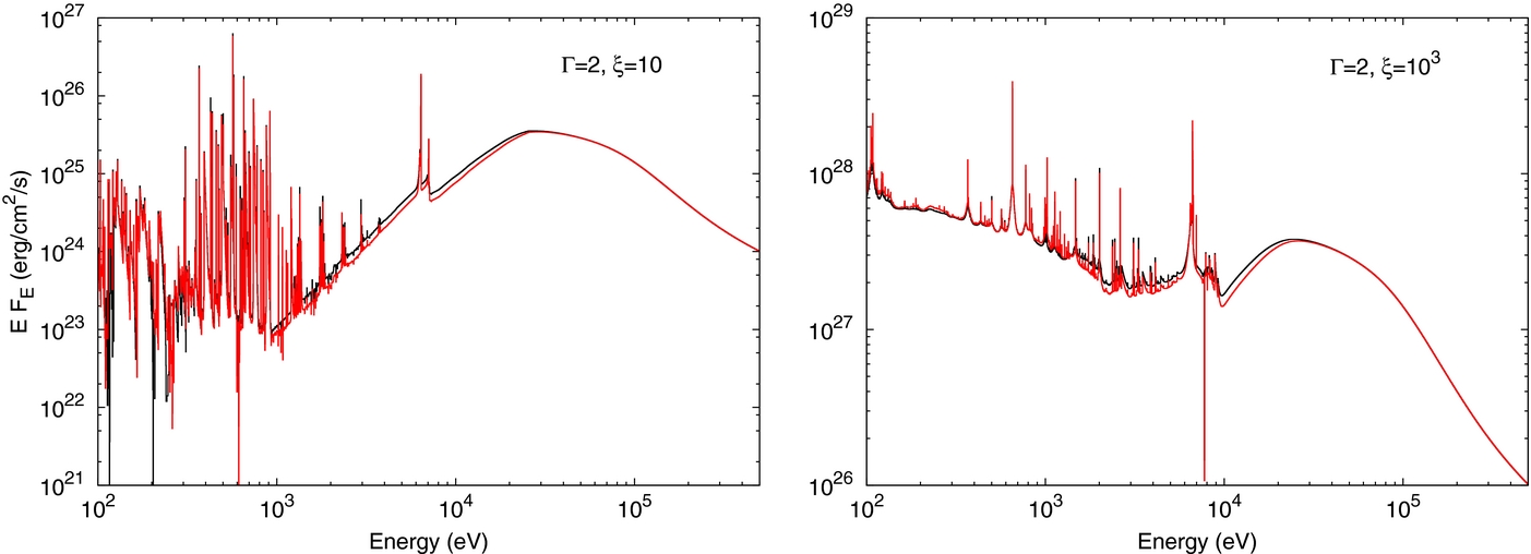
Figure 21. Comparison of the reflected spectra as calculated with xillver (black curve), reflionx (blue curve), and the Monte Carlo simulation (red curve), for an illumination with Γ = 2, ξ = 1, and solar abundances.
Download figure:
Standard image High-resolution image
As a bottom line, the differences between the MC simulation and either xillver or reflionx are not larger than 30%, which is reasonable given the simplistic approximation used in those models. However, this level of performance may not be adequate for the analysis of such current and future X-ray missions as NuSTAR (Harrison et al. 2010) and eROSITA (Predehl et al. 2011). Furthermore, the Compton-hump spectrum can provide important constraints on disk inclination. Therefore, our goal is to improve this aspect of the code in future versions of xillver.
4. CONCLUSIONS
In this paper, we have presented a new and complete library of synthetic spectra for modeling radiation that is reprocessed in an accretion disk and emitted as a reflected spectrum, which is generated in response to illumination by an incident power-law spectrum. This present version of our code xillver is an update of those presented in García & Kallman (2010) and García et al. (2011). We have made several improvements to both the routines and the atomic data and have produced a large grid of reflection models covering a wide range of parameters. Each model is characterized by the photon index Γ of the illuminating radiation, the ionization parameter ξ at the surface of the disk, and the Fe abundance with respect to its solar value. A total of 720 reflected spectra are provided in a single FITS file12 suitable for the analysis of X-rays observations via the atable model in xspec. In order to represent the physical conditions typically observed in most accreting sources, this library covers the following range of parameters: 1.2 ⩽ Γ ⩽ 3.4, 1 ⩽ ξ ⩽ 104, and 0.5 ⩽ AFe ⩽ 10.
The spectrum that illuminates the surface of the accretion disk is assumed to be a power law in the 10−1 to 106 eV energy range, with a sharp low-energy cutoff at 100 eV and an exponential high-energy cutoff at 300 keV. The low-energy cutoff is important for spectra with steep power laws (Γ > 2); it prevents the spectrum from being unphysically overpopulated with low-energy photons. The power law is extended up to 1 MeV because in the low-Γ case this portion of the spectrum is rich in high-energy photons, which importantly effect both the gas temperature and the reflected spectrum.
The intensity of the illuminating spectrum, which is specified by the ionization parameter ξ, significantly impacts the ionization structure of the gas. In all models, the gas temperature in the vertical direction has a similar profile. Near the surface, where the illumination is intense, there is a hot layer (T ≳ 106 K) where Compton heating and cooling dominate. At larger depths, a warm/cold region exists where photoelectric opacity and recombination dominate. The depth at which the transition between these two regimes occurs increases as ξ increase and as the incident spectrum softens (large Γ). Above the transition layer, the radiation field thermalizes and the gas temperature remains fairly constant at around 105 K. For low ionization (ξ ≲ 100–500), the reflected spectrum displays a very rich set of emission lines superimposed on a strongly absorbed continuum. For high ionization (ξ ≳ 500–1000), the spectrum consists of very narrow emission lines from ionized species and a continuum that resembles the incident power law.
We have presented detailed comparisons with the reflection models reflionx (Ross & Fabian 2005) and pexrav (Magdziarz & Zdziarski 1995). The reflionx model is more similar to ours because of its complexity and the range of physical processes considered. Furthermore, reflionx and xillver both characterize the illuminating spectrum as a power law, cover the same energy range, and use the same definition for the input parameters. The spectra generated by the two codes are in good agreement. The spectra agree best for large Γ (soft spectra) and low values of ξ. However, at low energies reflionx generates an excess of soft flux compared to xillver. For hard spectra, Γ = 1.4, and high ionization, ξ = 103, the difference in the continuum at 1 keV is about an order of magnitude. This large discrepancy is not well understood and requires further analysis.
At very high or very low ionization, xillver and reflionx predict similar EWs for the Fe K emission feature (including both Kα and Kβ), although the values for xillver are generally larger. However, at intermediate levels of ionization, in the 102 ≲ ξ ≲ 103 range, the two models disagree strongly: the Fe K EWs computed in this range computed using reflionx drop drastically. The effect is presumably because reflionx assumes that the Fe K lines from second-row ions are completely suppressed by Auger resonant destruction.
Comparing xillver with the more simplistic models pexrav and pexriv highlights the importance of performing detailed calculations which take into account key physical processes. The greatest deficiency of these models is that they do not generate emission lines. The neutral pexrav model is in reasonable agreement with xillver concerning the level of the continuum and the strength of the edges. However, for moderate or high ionization (ξ ≳ 20), the pexriv model is in strong disagreement because it assumes an isothermal disk, as previously pointed out by Fabian & Ross (2010).
The library of models presented in this paper is suitable for modeling the reflection spectra of accreting sources when the thermal disk component of emission is small compared to the incident power-law component. That is, the present version of xillver is suitable for analyzing the spectra of AGNs, and also GBHs in the hard state, when the disk component is cool and faint. For GBHs in the thermal or steep power-law states (Remillard & McClintock 2006), the strong thermal component entering the atmosphere from below will significantly change the ionization structure of the disk. In a future publication, we will report on an extension of xillver that is appropriate for modeling reflection spectra in the presence of a strong thermal component.
Regardless of how accurate xillver (or any such slab reflection model) becomes, it is by itself inadequate for modeling the reflection component in the spectra of accreting black holes. For example, current black hole spin determinations based on fitting of the Fe K line naively assume a single ionization state for the reflecting portion of the disk, which can extend over hundreds of gravitational radii. We plan to construct more realistic models for particular illumination geometries that allow for an ionization gradient in the radial direction. This work will combine the general relativistic approach implemented in the relline code (Dauser et al. 2010, 2013) with the model spectra presented in this paper.
Footnotes
- 6
- 7
- 8
- 9
- 10
- 11
- 12