


Abstract
We demonstrate the non-ergodicity of a simple Markovian stochastic process with space-dependent diffusion coefficient D(x). For power-law forms D(x) ≃ |x|α, this process yields anomalous diffusion of the form 〈x2(t)〉 ≃ t2/(2−α). Interestingly, in both the sub- and superdiffusive regimes we observe weak ergodicity breaking: the scaling of the time-averaged mean-squared displacement  remains linear in the lag time Δ and thus differs from the corresponding ensemble average 〈x2(t)〉. We analyse the non-ergodic behaviour of this process in terms of the time-averaged mean-squared displacement
  and its random features, i.e. the statistical distribution of
  and the ergodicity breaking parameters. The heterogeneous diffusion model represents an alternative approach to non-ergodic, anomalous diffusion that might be particularly relevant for diffusion in heterogeneous media.
Export citation and abstract BibTeX RIS

Content from this work may be used under the terms of the Creative Commons Attribution 3.0 licence. Any further distribution of this work must maintain attribution to the author(s) and the title of the work, journal citation and DOI.
Since the early systematic studies of Perrin and Nordlund [1], single particle tracking has become a routine method for tracing individual particles in microscopic systems [2], but also for animal [3] and human [4] motion patterns. In a wide range of systems and over many time and length scales, these measurements reveal anomalous diffusion with mean squared displacement (MSD) 〈x2(t)〉 ≃ tp [5]: subdiffusion (0 < p < 1) was found for the passive motion of tracers in living biological cells [6–11], a field in which single particle tracking has proved to be particularly useful, or for bacteria in biofilms [12]. A comprehensive review on anomalous diffusion in the crowded environment of living cells was recently published [13]. More generally, subdiffusion is observed in a large variety of systems, including charge carrier transport in amorphous semiconductors [14], tracer dispersion in groundwater [15] or in fractal systems [16, 17]. Superdiffusion (p > 1) is observed for active motion in the biological cells [11] of mussels [18], plant lice [19] or higher animals and humans [3, 4].
Given the broad use of single particle tracking methods to garner diffusion data in both micro- and macroscopic systems and thus the need to evaluate and physically interpret the recorded time series x(t) of the particle position, the ergodic properties of a stochastic process are of particular current interest: is the information obtained from time averages of a single or few trajectories representative for the ensemble? In other words, are sufficiently long time averages reproducible and equivalent to the corresponding ensemble averages [20, 21]? This question has motivated some vivid activity in the field of statistical physics recently. Thus, of the various stochastic models for anomalous diffusion, diffusion on random fractals has been shown to be ergodic [22]. Fractional Brownian and fractional Langevin equation motion driven by long-range correlated Gaussian noise are transiently non-ergodic [23–26]. In contrast, subdiffusive Scher–Montroll continuous time random walks (CTRW) [14, 27] with diverging characteristic waiting time exhibit weak ergodicity breaking [28], and time averages remain random even in the long time limit [29]. Weak ergodicity breaking was indeed observed for the blinking dynamics of quantum dots [30], protein motion in human cell walls [7], lipid granule diffusion in yeast cells [8] and of insulin granules in MIN6 cells [9].
While CTRW processes represent an elegant tool to describe anomalous diffusion, the occurrence of power-law distributed waiting times is far from universal. We therefore ask the question of whether we can create a simple, alternative stochastic model that still features this intricate, weakly non-ergodic behaviour. Here we show that the MSD of Markovian, heterogeneous diffusion processes (HDPs) with space dependent diffusion constant D(x) ≃ |x|α scales like 〈x2(t)〉 ≃ tp with p = 2/(2 − α), while the time averaged MSD  scales linearly in both sub- (α < 0) and superdiffusive (α > 0) regimes. We quantify the non-ergodicity in terms of the ergodicity breaking parameters and the amplitude scatter distribution of
  . We showcase the analogies and differences between HDPs and other non-ergodic diffusion processes.
Physically, a space dependent diffusivity appears a natural description for diffusion in heterogeneous systems. Examples include Richardson diffusion in turbulence [31] as well as mesoscopic approaches to transport in heterogenous porous media [32] and on random fractals [33]. Recently, maps of the local cytoplasmic diffusivities in bacterial and eukaryotic cells showed a highly heterogeneous landscape [34], recalling the strongly time-varying diffusion coefficients of tracers in cells, see e.g. [35].
1. Heterogeneous diffusion model
We start with the Markovian Langevin equation for the displacement x(t) of a test particle in a heterogeneous medium with space dependent diffusivity D(x), namely,
Here, ζ(t) is white Gaussian noise with δ-correlation 〈ζ(t)ζ(t')〉 = δ(t − t') and zero mean 〈ζ(t)〉 = 0. In the following we interpret the Langevin equation in the Stratonovich sense [36], to ensure the correct limiting transition for the noise with infinitely short correlation times [37]5. Specifically, for D(x) we employ the power-law form [38, 39]6

The dimension of D0 is [D0] = cm2−α s−1. In the Stratonovich interpretation, we introduce the substitution ![$y=\int ^x[2D(x')]^{ -1/2}\,\mathrm {d}x'$](https://content.cld.iop.org/journals/1367-2630/15/8/083039/revision1/nj475079ieqn6.gif) , where y(t) is the Wiener process [36]. For the initial condition P(x,0) = δ(x) a compressed (α < 0) or stretched (α > 0) Gaussian probability density function (PDF)
, where y(t) is the Wiener process [36]. For the initial condition P(x,0) = δ(x) a compressed (α < 0) or stretched (α > 0) Gaussian probability density function (PDF)

emerges (see appendix A), with p = 2/(2 − α). The ensemble averaged MSD  becomes

Thus, for α < 0 we find subdiffusion, and superdiffusion for α > 0. Brownian motion with 〈x2(t)〉 = 2D0t emerges for α = 0, and α = 1 produces ballistic motion. The diffusion becomes increasingly fast when α tends to 2.
Figure 1 compares the PDF (2) to simulations results (see below). Compared to the Gaussian shape of Brownian motion (α = 0), we observe a depletion in regions of higher diffusivity. For subdiffusion, this causes the central dip of the PDF, while for superdiffusion probability is shifted towards the origin. Note that the shape of the PDFs is significantly different from those of CTRW processes. In particular, for the subdiffusive case, the CTRW-PDF has a pronounced cusp at the origin [5]. Curiously, the subdiffusive shape in figure 1 resembles the propagator for retarded wave motion [40].

Figure 1. Time evolution of the PDF for sub- (left) and superdiffusion (right). We compare simulations results (full lines) to the analytical result (dashed) of equation (2) with D0 = 1. The small discrepancy is due to the rectified form of the diffusion coefficient at the origin implemented in simulations (see text).
Download figure:
Standard image High-resolution imageTo characterize the HDP, we calculate the position autocorrelation (see appendix A) for the case t2 > t1,
with the hypergeometric function 2F1(z). The Brownian limit 〈x(t)x(t + τ)〉 = 2D0t follows for α = 0, while for t1 = t2 we recover equation (3). The asymptotic behaviour of expression (4), 〈x(t)x(t + τ)〉 ≃ τ(p−1)/2t(p+1)/2 for τ/t ≫ 1 implies that the correlations decay with τ for subdiffusive processes whereas they increase in the case of superdiffusion, similar to fractional Brownian motion (FBM) [23]. We also obtain the correlation of two consecutive increments along x(t). For τ/t ≪ 1, we find the simple expressions for p = 1/2 and 2:

Indeed the occurrence of antipersistence (negative correlations) for subdiffusion and persistence for superdiffusion holds for all values of p (appendix A), again similar to FBM. We present exact results for the velocity autocorrelation function in appendix A.
To connect to single particle tracking experiments we now turn to the time averaged MSD of a trajectory x(t),

where Δ is the lag time and T the length of the time series x(t). In equation (6) we introduced the additional average over individual trajectories,  [29]. For Δ ≪ T we find the linear Δ-dependence (compare appendix B)

Remarkably, this result holds for both sub- and superdiffusive regimes, and we find the exact match
Equation (7) is our central result. Despite the simple nature of the Markovian HDP, we find that it displays weak non-ergodicity, i.e. the scaling of time and ensemble averages is different,  . Linear scaling of the type of equation (7) was found for subdiffusive CTRWs [29], but also for correlated CTRWs [41], ageing, non-renewal CTRW processes [42] and time-scaled Brownian motion [43]. It contrasts the ultraweak non-ergodicity of superdiffusive CTRWs [44]. In particular, the dependence on the length T of the time series is identical to CTRW and correlated CTRW subdiffusion: with increasing T the effective diffusivity Deff ≃ Tp−1 decreases. In the superdiffusive regime, this Deff increases with time, the particle becomes more mobile. For HDP processes the ageing dependence on T arises when the particle continues to venture into regions of changing diffusivities, for subdiffusive CTRWs this is due to increasingly longer sojourn times.
Exploring HDPs in more detail numerically, we note that the Langevin equation in the Stratonovich interpretation leads to an implicit mid-point iterative scheme for the particle displacement. At step i + 1, we thus have ![$x_{i+1}-x_i=\sqrt {2D([x_{i+1}+x_i]/2)}(y_{i+1}-y_{i})$](https://content.cld.iop.org/journals/1367-2630/15/8/083039/revision1/nj475079ieqn10.gif) , where the increments (yi+1 − yi) of the Wiener process represent a δ-correlated Gaussian noise with unit variance. Unit time intervals separate consecutive iteration steps. In our numerical study we consider the two generic cases p = 1/2 and 2. To avoid divergencies in the discrete scheme, for subdiffusion we regularize the diffusivity at x = 0, choosing D(x) = D0A/(A + x2), such that for x2 ≫ A we recover the original relation (1). For superdiffusion, to avoid trapping at x = 0 and thus prohibitively expensive simulations, we use the shifted form D(x) = D0(|x| + 1), again with the correct scaling for large |x|.
, where the increments (yi+1 − yi) of the Wiener process represent a δ-correlated Gaussian noise with unit variance. Unit time intervals separate consecutive iteration steps. In our numerical study we consider the two generic cases p = 1/2 and 2. To avoid divergencies in the discrete scheme, for subdiffusion we regularize the diffusivity at x = 0, choosing D(x) = D0A/(A + x2), such that for x2 ≫ A we recover the original relation (1). For superdiffusion, to avoid trapping at x = 0 and thus prohibitively expensive simulations, we use the shifted form D(x) = D0(|x| + 1), again with the correct scaling for large |x|.
2. Numerical results
From the generated trajectories, we compute the PDF (figure 1) as well as the ensemble and time averaged MSDs. The MSDs are shown in figure 2. For the ensemble averaged MSD (blue curve) we observe excellent agreement with equation (3). In the subdiffusion case, the predicted behaviour (3) is reached after less than a dozen steps, such that the rectification of D(x) and the choice of the off-centre initial position x0 are practically negligible. For superdiffusion, an extended region of almost normal diffusion is observed for small particle displacements, as long as |x| < 1 in the rectified D(x). The long time behaviour shows good agreement between theory and simulations. The time averaged MSDs and their mean  follow nicely the predicted linear scaling. Only when the lag time Δ approaches T the linear behaviour levels off due to the finite trajectory length T.
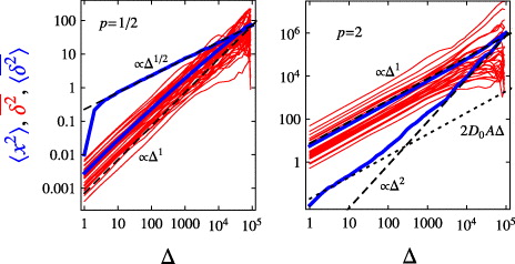
Figure 2. Ensemble and time averaged MSDs for sub- and superdiffusive HDPs for T = 105, D0 = 1 and A = 0.01. The thin red lines show results for individual time averaged trajectories, the thick blue lines refer to the ensemble averaged MSD 〈x2(t)〉 and the trajectory average  of the time averaged MSD. The expected results (3) and (7) are shown by dashed lines. The time averaged MSDs are logarithmically sampled. The initial position is x0 = 0.1 for all trajectories. For subdiffusion, the discrepancy of theory and simulated results for
  is due to the D(x) rectification, see text.
Download figure:
Standard image High-resolution imageNext we study the apparent diffusion coefficients and scaling exponents from the individual  . The points of each trace
  were logarithmically binned. The initial part of the trajectory, Δ = 1–102 steps, was fitted by a linear law with diffusivity D1. The long-time regime, Δ ∼ 102–104 steps, was fitted with two parameters,
  . The distributions of D1, Dβ and β were then fitted with the three-parameter gamma distribution, g(z) ∼ zν−1 e−z/b e−a/z, the parameters being fixed by the first three moments obtained from the histograms. This gamma distribution was recently proposed for the spread with Δ of
  of a Brownian walker [45]. In addition, we extracted the amplitude scatter PDF
  of individual
  around the mean
  .
.
Figures 3 and 4 show the results of this analysis, together with the fits to the gamma distribution, g(z). We see that the amplitude scatter shows a pronounced spread around the ergodic value ξ = 1 in both sub- and superdiffusive regimes. The shape of ϕ(ξ) changes only marginally with Δ in the linear region of  . Broad distributions of ϕ(ξ) are known from both sub- and superdiffusive CTRWs. The differences are, however, that for subdiffusive CTRWs ϕ(ξ) has a finite value at ξ = 0 due to completely immobilized particles [29]. For superdiffusive CTRWs ϕ(ξ) decays to zero at ξ = 0, but changes significantly with Δ [44]. The scatter distribution ϕ(ξ) is thus a good criterion to distinguish HDPs and CTRWs.
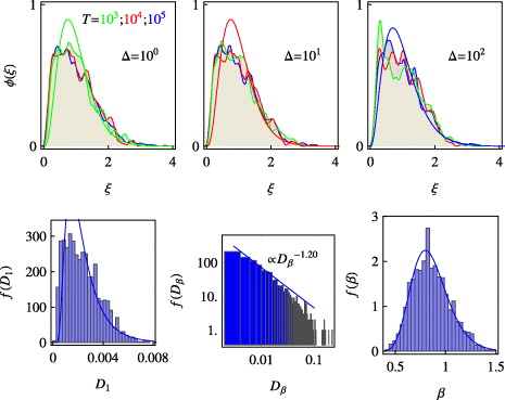
Figure 3. Amplitude scatter PDF ϕ(ξ) for subdiffusive HDP (top) and distributions of the fit parameters D1, Dβ and β (bottom). Parameters Δ and T are indicated in the panels. In the upper panel the red, green and blue curves denote the same trace lengths as in figure 1. The shaded histograms are the simulations results shown simultaneously for three T values. The curves are the Gamma-distributions shown in every of the upper panels for one trace length T only, with the corresponding colour. Solid envelopes are three-parameter fits to g(z) (see text). At least 103 trajectories were analysed for each T, with T = 105.
Download figure:
Standard image High-resolution image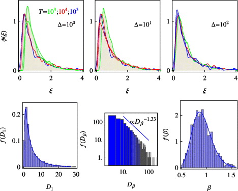
Figure 4. The same as in figure 3 but for superdiffusive HDPs.
Download figure:
Standard image High-resolution imageMore specifically, for subdiffusion the distributions of D1 and the amplitude scatter ϕ(ξ) are wider, while for superdiffusion they show a sharper peak with a maximum shifted to the mean at ξ = 1. The width of ϕ(ξ) is roughly unity for subdiffusion and 1/2 for superdiffusion. It changes only slightly with T in the range T = 103–105, see figure 3. The distributions for Dβ typically exhibit a long power-law tail with f(Dβ) ∼ D−1.2...1.4β. The distributions for the apparent long-time exponent β are similar for sub- and superdiffusion, with 〈β〉p=1/2 ≈ 0.86 and 〈β〉p=2 ≈ 0.92. Finite T-effects lead to the undershoot of 〈β〉 compared to the theoretical value of unity.
Consider now the ergodicity breaking parameter [29]
that provides a good measure for the dispersion of time averaged MSDs for different types of diffusion processes [46]. The sufficient condition of ergodicity of a process is EB = 0. A necessary condition is that the ratio of the time and ensemble averaged MSD equals unity. Here we observe that this condition is not fulfilled for p ≠ 1,
The ergodicity breaking parameters EB and  extracted from simulations data at Δ/T ≪ 1 is EB ≈ 0.4 for sub- and EB ≈ 1.4 for superdiffusion, indicating the weakly non-ergodic nature of HDP processes in both regimes. The parameter
  follows the predicted scaling for large Δ and T values, i.e. when both ensemble and time averaged MSDs have converged to the theoretical scaling (figures 2 and 5). For Brownian diffusion our simulations yield the correct finite-time scaling
  and sharp amplitude scatter ϕ(ξ) ∼ δ(ξ − 1) at T → ∞, indicating the ergodic behaviour for long traces and the self-averaging property of normal diffusion. For p = 2 at Δ/T → 0 the estimated theoretical value is EB = 2/3 (equation (C.1)) close to the value from simulations.

Figure 5. Ergodicity breaking parameters  (thick) and EB (thin blue curves) as obtained from simulations (T = 105). The theoretical asymptotes for
  (left panel, dashed lines) and approximate equation (C.1) for EB (right panel, see appendix C).
Download figure:
Standard image High-resolution imageThe simulations show that for subdiffusion,  increases with Δ/T, while for superdiffusion it decreases with Δ/T (figure 5). In both cases
  approaches unity as Δ → T. At Δ/T ≪ 1,
  for p < 1 assumes smaller values, indicating weaker deviations from ergodicity, in contrast to superdiffusion, see figure 5. The parameter EB defined via the fourth moment is overall a more robust characteristic of the process. For instance, it varies only slightly with T and Δ for Δ/T ≪ 1 (not shown).
3. Conclusions
Anomalous diffusion is a widely observed phenomenon across many scales and disciplines. Following the dramatic increase of single particle tracking studies, the question arises of how we can physically interpret the recorded trajectories in terms of time averages of observables such as the MSD. Namely, in most cases the available physical theories provide results for the ensemble averages of physical observables. Once a system exhibits weak ergodicity breaking, however, the inequivalence of ensemble from time averages prohibits the application of such ensemble theories to the measured, time-averaged quantities. The quantitative interpretation of time averages therefore requires knowledge about whether the system is ergodic and the standard results can be used to fit the data, or whether the system is weakly non-ergodic. In that case knowledge of the time averaged observables is indispensable.
Here we discussed the seemingly simple Markovian HDP with power-law space-dependent diffusion coefficient, defined in terms of a Langevin equation, which is fully local in both space and time. Despite this locality HDPs are weakly non-ergodic: the time averaged MSD  scales linearly with the lag time Δ for both sub- and superdiffusion. Such a behaviour was previously known for subdiffusion from more complex processes: CTRWs with diverging characteristic waiting time [29], CTRWs with correlated waiting times [41], non-renewal, ageing CTRWs [42] and time-scaled Brownian motion [43]. For superdiffusion only an ultraweak ergodicity breaking was reported in which the coefficients of the time and ensemble MSDs differ [44], while space-correlated CTRWs feature a Richardson-type hyperdiffusive scaling of the time averaged MSD [41].
The amplitudes of  of different trajectories show a broad and asymmetric distribution, another sign of non-ergodicity. In contrast to CTRW subdiffusion, however, in HDPs there is no contribution from completely immobile trajectories. Concurrently, HDPs exhibit (anti)persistence of the increment correlation functions, such that for subdiffusion (superdiffusion) subsequent increments preferentially have opposite (equal) direction. This property is similar to the noise correlator of FBM, moreover the velocity autocorrelator of both HDP and FBM processes is strikingly similar.
HDPs represent new tools for the description of weakly non-ergodic dynamics. Due to their intuitive formulation in terms of space-dependent diffusivities this dynamic behaviour of HDPs directly follows from the physical properties of the environment. HDPs may be distinguished from other processes due to the difference in the amplitude scatter distribution of time averaged MSDs, the increment autocorrelation function, as well as the two ergodicity breaking parameters. It will be interesting to see whether two-dimensional generalizations of the HDP model may grasp some of the interesting dynamical patterns observed in single particle motion in biological cells.
How general are the results obtained herein for power-law forms of the position dependent diffusion coefficient? A preliminary numerical analysis shows that similar forms of weak ergodicity breaking is observed when we consider diffusivities with both stronger and weaker x-dependence, for instance, exponential or logarithmic forms. Details will be presented in a separate publication.
Acknowledgments
We thank E Barkai and H Buening for discussions and acknowledge funding from the Academy of Finland (FiDiPro scheme to RM) and Deutsche Forschungsgemeinschaft (grant no. CH 707/5-1 to AGC).
Appendix A.: Probability density function
To solve the Langevin equation  in the Stratonovich sense we introduce the new variable [36]

where y(t) is the Wiener process with the known Gaussian PDF for the initial condition y(0) = 0, namely,

Returning to the x-variable yields the PDF (2).
With the back-transformation y → x, from equation (A.1) we find that x(t) = 2p/2p−p|y|psign(y), and the autocorrelation function is evaluated via the two-point PDF for the Wiener process

where we used the transition probability

Evaluating the integral in equation (A.3) we arrive at equation (4).
Appendix B.: Time averages
To obtain the time averaged MSD, we calculate the auxiliary integral

To this end, we use the representation of the hypergeometric function via the Fox H-function (see [47], equation (1.131)) and then employ the integral over the H-function following [48], equation (8.3.2.7), arriving at
Finally, we use [48], equation (8.3.2.3)] to find the result for the time averaged MSD, equation (7).
Appendix C.: Approximative scheme for the EB parameter
We now outline an approximative scheme to evaluate the ergodicity breaking parameter EB. Namely, from equation (A.1) we express the particle displacement through |x(t)| ∼ |y(t)|p, where y(t) is the Wiener process. Then, we take 〈x2(t)〉 = (2D0tp−2)p, which at Δ/T ≪ 1 yields  . Thus
  , identical to the result in the main text derived from the exact approach (A.1). The fourth moment of the time averaged MSD in this approximative scheme becomes

involving a combination of altogether nine terms, each containing a product of four noise terms ζ(t). Using 〈ζ(t1)ζ(t2)ζ(t3)ζ(t4)〉 = δ(t1 − t2)δ(t3 − t4) + δ(t1 − t3)δ(t2 − t4) + δ(t1 − t4)δ(t2 − t3), the integrals from the Wiener processes disappear and two integrations are left. These were evaluated numerically for a given value of p to extract the scaling of the ergodicity breaking parameter
for Δ/T ≪ 1. Using the result  , we expand the fourth moment up to Δ2 to compute EB(Δ/T → 0), corresponding to the limit T → ∞. For Brownian motion (p = 1) we find the correct scaling EB = (4/3)(Δ/T). The scheme for HDPs with p = 2 yields EB(0) = 2/3, close to the simulations results. Overall, this approximative scheme predicts that EB grows as the system deviates from the ergodic state p = 1 for both sub- and superdiffusion, see figure 5.
Appendix D.: Velocity autocorrelations
We now determine the normalized velocity autocorrelation function

With the position autocorrelations (4), C(δ)v(τ) becomes a universal function of δ/τ. C(δ)v(τ) is plotted in figure C.1. Thus, for superdiffusion the correlations remain positive, for subdiffusion C(δ)v(τ) features a negative region mirroring the anti-persistence of the motion. In figure C.1 we also show the complete decay of the correlations within the increment δ for Brownian motion. Moreover, we include the velocity autocorrelation function of FBM for the sub- and superdiffusive cases. The general behaviours are quite similar.

Figure C.1. Normalized velocity autocorrelation function C(δ)v(τ) for sub- and superdiffusion (dashed lines). The dotted curve corresponds to uncorrelated Brownian motion (p = 1), and the solid green curves represent FBM with the indicated Hurst coefficients (in the MSD, p = 2H).
Download figure:
Standard image High-resolution image